class: top, center, title-slide # Single Case Experimental Design #2 ## A workshop for routine clinicians - Day 2: Analysing time series data ### University of Sheffield - Clinical and Applied Psychology Unit --- class: center, middle, split-three, about-me-slide background-image: url(uos.png), url(pearls.jpg) background-position:5% 95%, 98% 96% background-size: 110px 50px, 10% .column.bg-main1[.content[ <img style="border-radius: 50%;" src="https://catalyse.uk.com/wp-content/uploads/sites/3/2015/10/SKcrop.jpg" width="150px"/> ### Steve Kellett #### Clinical Psychologist .fade[Sheffied Health & Social Care NHS Foundation Trust] [<svg viewBox="0 0 512 512" style="position:relative;display:inline-block;top:.1em;height:1.5em;" xmlns="http://www.w3.org/2000/svg"> <path d="M464 64H48C21.49 64 0 85.49 0 112v288c0 26.51 21.49 48 48 48h416c26.51 0 48-21.49 48-48V112c0-26.51-21.49-48-48-48zm0 48v40.805c-22.422 18.259-58.168 46.651-134.587 106.49-16.841 13.247-50.201 45.072-73.413 44.701-23.208.375-56.579-31.459-73.413-44.701C106.18 199.465 70.425 171.067 48 152.805V112h416zM48 400V214.398c22.914 18.251 55.409 43.862 104.938 82.646 21.857 17.205 60.134 55.186 103.062 54.955 42.717.231 80.509-37.199 103.053-54.947 49.528-38.783 82.032-64.401 104.947-82.653V400H48z"></path></svg>](mailto:s.kellett@sheffield.ac.uk) [<svg viewBox="0 0 448 512" style="position:relative;display:inline-block;top:.1em;height:1.5em;" xmlns="http://www.w3.org/2000/svg"> <path d="M0 32v448h448V32H0zm262.2 334.4c-6.6 3-33.2 6-50-14.2-9.2-10.6-25.3-33.3-42.2-63.6-8.9 0-14.7 0-21.4-.6v46.4c0 23.5 6 21.2 25.8 23.9v8.1c-6.9-.3-23.1-.8-35.6-.8-13.1 0-26.1.6-33.6.8v-8.1c15.5-2.9 22-1.3 22-23.9V225c0-22.6-6.4-21-22-23.9V193c25.8 1 53.1-.6 70.9-.6 31.7 0 55.9 14.4 55.9 45.6 0 21.1-16.7 42.2-39.2 47.5 13.6 24.2 30 45.6 42.2 58.9 7.2 7.8 17.2 14.7 27.2 14.7v7.3zm22.9-135c-23.3 0-32.2-15.7-32.2-32.2V167c0-12.2 8.8-30.4 34-30.4s30.4 17.9 30.4 17.9l-10.7 7.2s-5.5-12.5-19.7-12.5c-7.9 0-19.7 7.3-19.7 19.7v26.8c0 13.4 6.6 23.3 17.9 23.3 14.1 0 21.5-10.9 21.5-26.8h-17.9v-10.7h30.4c0 20.5 4.7 49.9-34 49.9zm-116.5 44.7c-9.4 0-13.6-.3-20-.8v-69.7c6.4-.6 15-.6 22.5-.6 23.3 0 37.2 12.2 37.2 34.5 0 21.9-15 36.6-39.7 36.6z"></path></svg>](https://www.researchgate.net/profile/Stephen-Kellett) ]] .column.bg-main2[.content[ <img style="border-radius: 50%;" src="https://pbs.twimg.com/profile_images/1235537191683723265/Qo6rZ317_400x400.jpg" width="150px"/> ### Mel Simmonds-Buckley #### Researcher .fade[University of Sheffield] [<svg viewBox="0 0 512 512" style="position:relative;display:inline-block;top:.1em;height:1.5em;" xmlns="http://www.w3.org/2000/svg"> <path d="M464 64H48C21.49 64 0 85.49 0 112v288c0 26.51 21.49 48 48 48h416c26.51 0 48-21.49 48-48V112c0-26.51-21.49-48-48-48zm0 48v40.805c-22.422 18.259-58.168 46.651-134.587 106.49-16.841 13.247-50.201 45.072-73.413 44.701-23.208.375-56.579-31.459-73.413-44.701C106.18 199.465 70.425 171.067 48 152.805V112h416zM48 400V214.398c22.914 18.251 55.409 43.862 104.938 82.646 21.857 17.205 60.134 55.186 103.062 54.955 42.717.231 80.509-37.199 103.053-54.947 49.528-38.783 82.032-64.401 104.947-82.653V400H48z"></path></svg>](mailto:m.simmonds-buckley@sheffield.ac.uk) [<svg viewBox="0 0 640 512" style="position:relative;display:inline-block;top:.1em;height:1.5em;" xmlns="http://www.w3.org/2000/svg"> <path d="M622.34 153.2L343.4 67.5c-15.2-4.67-31.6-4.67-46.79 0L17.66 153.2c-23.54 7.23-23.54 38.36 0 45.59l48.63 14.94c-10.67 13.19-17.23 29.28-17.88 46.9C38.78 266.15 32 276.11 32 288c0 10.78 5.68 19.85 13.86 25.65L20.33 428.53C18.11 438.52 25.71 448 35.94 448h56.11c10.24 0 17.84-9.48 15.62-19.47L82.14 313.65C90.32 307.85 96 298.78 96 288c0-11.57-6.47-21.25-15.66-26.87.76-15.02 8.44-28.3 20.69-36.72L296.6 284.5c9.06 2.78 26.44 6.25 46.79 0l278.95-85.7c23.55-7.24 23.55-38.36 0-45.6zM352.79 315.09c-28.53 8.76-52.84 3.92-65.59 0l-145.02-44.55L128 384c0 35.35 85.96 64 192 64s192-28.65 192-64l-14.18-113.47-145.03 44.56z"></path></svg>](https://scholar.google.com/citations?user=T85W7TYAAAAJ&hl=en) [<svg viewBox="0 0 448 512" style="position:relative;display:inline-block;top:.1em;height:1.5em;" xmlns="http://www.w3.org/2000/svg"> <path d="M0 32v448h448V32H0zm262.2 334.4c-6.6 3-33.2 6-50-14.2-9.2-10.6-25.3-33.3-42.2-63.6-8.9 0-14.7 0-21.4-.6v46.4c0 23.5 6 21.2 25.8 23.9v8.1c-6.9-.3-23.1-.8-35.6-.8-13.1 0-26.1.6-33.6.8v-8.1c15.5-2.9 22-1.3 22-23.9V225c0-22.6-6.4-21-22-23.9V193c25.8 1 53.1-.6 70.9-.6 31.7 0 55.9 14.4 55.9 45.6 0 21.1-16.7 42.2-39.2 47.5 13.6 24.2 30 45.6 42.2 58.9 7.2 7.8 17.2 14.7 27.2 14.7v7.3zm22.9-135c-23.3 0-32.2-15.7-32.2-32.2V167c0-12.2 8.8-30.4 34-30.4s30.4 17.9 30.4 17.9l-10.7 7.2s-5.5-12.5-19.7-12.5c-7.9 0-19.7 7.3-19.7 19.7v26.8c0 13.4 6.6 23.3 17.9 23.3 14.1 0 21.5-10.9 21.5-26.8h-17.9v-10.7h30.4c0 20.5 4.7 49.9-34 49.9zm-116.5 44.7c-9.4 0-13.6-.3-20-.8v-69.7c6.4-.6 15-.6 22.5-.6 23.3 0 37.2 12.2 37.2 34.5 0 21.9-15 36.6-39.7 36.6z"></path></svg>](https://www.researchgate.net/profile/Mel-Simmonds-Buckley) ]] .column.bg-main3[.content[ <img style="border-radius: 50%;" src="https://pbs.twimg.com/profile_images/1434417640920002563/ZS62zhXl_400x400.jpg" width="150px"/> ### Chris Gaskell #### Clinical Psychologist .fade[Salford Royal NHS Foundation Trust] [<svg viewBox="0 0 512 512" style="position:relative;display:inline-block;top:.1em;height:1.5em;" xmlns="http://www.w3.org/2000/svg"> <path d="M459.37 151.716c.325 4.548.325 9.097.325 13.645 0 138.72-105.583 298.558-298.558 298.558-59.452 0-114.68-17.219-161.137-47.106 8.447.974 16.568 1.299 25.34 1.299 49.055 0 94.213-16.568 130.274-44.832-46.132-.975-84.792-31.188-98.112-72.772 6.498.974 12.995 1.624 19.818 1.624 9.421 0 18.843-1.3 27.614-3.573-48.081-9.747-84.143-51.98-84.143-102.985v-1.299c13.969 7.797 30.214 12.67 47.431 13.319-28.264-18.843-46.781-51.005-46.781-87.391 0-19.492 5.197-37.36 14.294-52.954 51.655 63.675 129.3 105.258 216.365 109.807-1.624-7.797-2.599-15.918-2.599-24.04 0-57.828 46.782-104.934 104.934-104.934 30.213 0 57.502 12.67 76.67 33.137 23.715-4.548 46.456-13.32 66.599-25.34-7.798 24.366-24.366 44.833-46.132 57.827 21.117-2.273 41.584-8.122 60.426-16.243-14.292 20.791-32.161 39.308-52.628 54.253z"></path></svg> ](https://twitter.com/chrisgaskell92) [<svg viewBox="0 0 496 512" style="position:relative;display:inline-block;top:.1em;height:1.5em;" xmlns="http://www.w3.org/2000/svg"> <path d="M165.9 397.4c0 2-2.3 3.6-5.2 3.6-3.3.3-5.6-1.3-5.6-3.6 0-2 2.3-3.6 5.2-3.6 3-.3 5.6 1.3 5.6 3.6zm-31.1-4.5c-.7 2 1.3 4.3 4.3 4.9 2.6 1 5.6 0 6.2-2s-1.3-4.3-4.3-5.2c-2.6-.7-5.5.3-6.2 2.3zm44.2-1.7c-2.9.7-4.9 2.6-4.6 4.9.3 2 2.9 3.3 5.9 2.6 2.9-.7 4.9-2.6 4.6-4.6-.3-1.9-3-3.2-5.9-2.9zM244.8 8C106.1 8 0 113.3 0 252c0 110.9 69.8 205.8 169.5 239.2 12.8 2.3 17.3-5.6 17.3-12.1 0-6.2-.3-40.4-.3-61.4 0 0-70 15-84.7-29.8 0 0-11.4-29.1-27.8-36.6 0 0-22.9-15.7 1.6-15.4 0 0 24.9 2 38.6 25.8 21.9 38.6 58.6 27.5 72.9 20.9 2.3-16 8.8-27.1 16-33.7-55.9-6.2-112.3-14.3-112.3-110.5 0-27.5 7.6-41.3 23.6-58.9-2.6-6.5-11.1-33.3 2.6-67.9 20.9-6.5 69 27 69 27 20-5.6 41.5-8.5 62.8-8.5s42.8 2.9 62.8 8.5c0 0 48.1-33.6 69-27 13.7 34.7 5.2 61.4 2.6 67.9 16 17.7 25.8 31.5 25.8 58.9 0 96.5-58.9 104.2-114.8 110.5 9.2 7.9 17 22.9 17 46.4 0 33.7-.3 75.4-.3 83.6 0 6.5 4.6 14.4 17.3 12.1C428.2 457.8 496 362.9 496 252 496 113.3 383.5 8 244.8 8zM97.2 352.9c-1.3 1-1 3.3.7 5.2 1.6 1.6 3.9 2.3 5.2 1 1.3-1 1-3.3-.7-5.2-1.6-1.6-3.9-2.3-5.2-1zm-10.8-8.1c-.7 1.3.3 2.9 2.3 3.9 1.6 1 3.6.7 4.3-.7.7-1.3-.3-2.9-2.3-3.9-2-.6-3.6-.3-4.3.7zm32.4 35.6c-1.6 1.3-1 4.3 1.3 6.2 2.3 2.3 5.2 2.6 6.5 1 1.3-1.3.7-4.3-1.3-6.2-2.2-2.3-5.2-2.6-6.5-1zm-11.4-14.7c-1.6 1-1.6 3.6 0 5.9 1.6 2.3 4.3 3.3 5.6 2.3 1.6-1.3 1.6-3.9 0-6.2-1.4-2.3-4-3.3-5.6-2z"></path></svg>](https://github.com/chris-gaskell) [<svg viewBox="0 0 512 512" style="position:relative;display:inline-block;top:.1em;height:1.5em;" xmlns="http://www.w3.org/2000/svg"> <path d="M464 64H48C21.49 64 0 85.49 0 112v288c0 26.51 21.49 48 48 48h416c26.51 0 48-21.49 48-48V112c0-26.51-21.49-48-48-48zm0 48v40.805c-22.422 18.259-58.168 46.651-134.587 106.49-16.841 13.247-50.201 45.072-73.413 44.701-23.208.375-56.579-31.459-73.413-44.701C106.18 199.465 70.425 171.067 48 152.805V112h416zM48 400V214.398c22.914 18.251 55.409 43.862 104.938 82.646 21.857 17.205 60.134 55.186 103.062 54.955 42.717.231 80.509-37.199 103.053-54.947 49.528-38.783 82.032-64.401 104.947-82.653V400H48z"></path></svg>](mailto:chris-gaskell@hotmail.co.uk) [<svg viewBox="0 0 640 512" style="position:relative;display:inline-block;top:.1em;height:1.5em;" xmlns="http://www.w3.org/2000/svg"> <path d="M622.34 153.2L343.4 67.5c-15.2-4.67-31.6-4.67-46.79 0L17.66 153.2c-23.54 7.23-23.54 38.36 0 45.59l48.63 14.94c-10.67 13.19-17.23 29.28-17.88 46.9C38.78 266.15 32 276.11 32 288c0 10.78 5.68 19.85 13.86 25.65L20.33 428.53C18.11 438.52 25.71 448 35.94 448h56.11c10.24 0 17.84-9.48 15.62-19.47L82.14 313.65C90.32 307.85 96 298.78 96 288c0-11.57-6.47-21.25-15.66-26.87.76-15.02 8.44-28.3 20.69-36.72L296.6 284.5c9.06 2.78 26.44 6.25 46.79 0l278.95-85.7c23.55-7.24 23.55-38.36 0-45.6zM352.79 315.09c-28.53 8.76-52.84 3.92-65.59 0l-145.02-44.55L128 384c0 35.35 85.96 64 192 64s192-28.65 192-64l-14.18-113.47-145.03 44.56z"></path></svg>](https://scholar.google.com/citations?user=gQuNwfYAAAAJ&hl=en&authuser=1&oi=ao) [<svg viewBox="0 0 448 512" style="position:relative;display:inline-block;top:.1em;height:1.5em;" xmlns="http://www.w3.org/2000/svg"> <path d="M0 32v448h448V32H0zm262.2 334.4c-6.6 3-33.2 6-50-14.2-9.2-10.6-25.3-33.3-42.2-63.6-8.9 0-14.7 0-21.4-.6v46.4c0 23.5 6 21.2 25.8 23.9v8.1c-6.9-.3-23.1-.8-35.6-.8-13.1 0-26.1.6-33.6.8v-8.1c15.5-2.9 22-1.3 22-23.9V225c0-22.6-6.4-21-22-23.9V193c25.8 1 53.1-.6 70.9-.6 31.7 0 55.9 14.4 55.9 45.6 0 21.1-16.7 42.2-39.2 47.5 13.6 24.2 30 45.6 42.2 58.9 7.2 7.8 17.2 14.7 27.2 14.7v7.3zm22.9-135c-23.3 0-32.2-15.7-32.2-32.2V167c0-12.2 8.8-30.4 34-30.4s30.4 17.9 30.4 17.9l-10.7 7.2s-5.5-12.5-19.7-12.5c-7.9 0-19.7 7.3-19.7 19.7v26.8c0 13.4 6.6 23.3 17.9 23.3 14.1 0 21.5-10.9 21.5-26.8h-17.9v-10.7h30.4c0 20.5 4.7 49.9-34 49.9zm-116.5 44.7c-9.4 0-13.6-.3-20-.8v-69.7c6.4-.6 15-.6 22.5-.6 23.3 0 37.2 12.2 37.2 34.5 0 21.9-15 36.6-39.7 36.6z"></path></svg>](https://www.researchgate.net/profile/Chris-Gaskell-2) ]] --- class: center, top, split-three, inverse background-image: url(https://rin.org.uk/resource/resmgr/nav21/nav21_map.png) background-position:8% 70% background-size: 375px 300px .column.bg-main1[.content[.right[ <img style="border-radius: 50%;" src=" " width="150px"/> # <svg viewBox="0 0 496 512" style="position:relative;display:inline-block;top:.1em;fill:var(--my-yellow);height:1em;" xmlns="http://www.w3.org/2000/svg"> <path d="M347.94 129.86L203.6 195.83a31.938 31.938 0 0 0-15.77 15.77l-65.97 144.34c-7.61 16.65 9.54 33.81 26.2 26.2l144.34-65.97a31.938 31.938 0 0 0 15.77-15.77l65.97-144.34c7.61-16.66-9.54-33.81-26.2-26.2zm-77.36 148.72c-12.47 12.47-32.69 12.47-45.16 0-12.47-12.47-12.47-32.69 0-45.16 12.47-12.47 32.69-12.47 45.16 0 12.47 12.47 12.47 32.69 0 45.16zM248 8C111.03 8 0 119.03 0 256s111.03 248 248 248 248-111.03 248-248S384.97 8 248 8zm0 448c-110.28 0-200-89.72-200-200S137.72 56 248 56s200 89.72 200 200-89.72 200-200 200z"></path></svg> Navigating these slides ]]] -- .column.bg-main2[.content[ <img style="border-radius: 50%;" src=" " width="150px"/> .Large[.bold[ ### Day 1 Aims + Intro Why Measures Designs Setting it up] ]]] -- .column.bg-main3[.content[ <img style="border-radius: 50%;" src=" " width="150px"/> .Large[.Bold[ ### Day 2 .bold[ [Analysis](#analysis-slide) [Practice](#practice-slide) <a href="https://sced-for-clinicians.netlify.app/resources/">Resources</a> ] ]]]] -- .footnote[.Large[**Note**: all underlined .white[.underline[white]] and .my-hot-white[.my-red[.underline[red]]] text are hyperlinks!] ] --- name: contents-slide class: inverse background-image: background-position: background-size: # <svg viewBox="0 0 496 512" style="position:relative;display:inline-block;top:.1em;fill:var(--my-yellow);height:1em;" xmlns="http://www.w3.org/2000/svg"> <path d="M347.94 129.86L203.6 195.83a31.938 31.938 0 0 0-15.77 15.77l-65.97 144.34c-7.61 16.65 9.54 33.81 26.2 26.2l144.34-65.97a31.938 31.938 0 0 0 15.77-15.77l65.97-144.34c7.61-16.66-9.54-33.81-26.2-26.2zm-77.36 148.72c-12.47 12.47-32.69 12.47-45.16 0-12.47-12.47-12.47-32.69 0-45.16 12.47-12.47 32.69-12.47 45.16 0 12.47 12.47 12.47 32.69 0 45.16zM248 8C111.03 8 0 119.03 0 256s111.03 248 248 248 248-111.03 248-248S384.97 8 248 8zm0 448c-110.28 0-200-89.72-200-200S137.72 56 248 56s200 89.72 200 200-89.72 200-200 200z"></path></svg> Navigating these slides <svg viewBox="0 0 576 512" style="position:relative;display:inline-block;top:.1em;fill:var(--my-yellow);height:1em;" xmlns="http://www.w3.org/2000/svg"> <path d="M528 64H48C21.49 64 0 85.49 0 112v288c0 26.51 21.49 48 48 48h480c26.51 0 48-21.49 48-48V112c0-26.51-21.49-48-48-48zm8 336c0 4.411-3.589 8-8 8H48c-4.411 0-8-3.589-8-8V112c0-4.411 3.589-8 8-8h480c4.411 0 8 3.589 8 8v288zM170 270v-28c0-6.627-5.373-12-12-12h-28c-6.627 0-12 5.373-12 12v28c0 6.627 5.373 12 12 12h28c6.627 0 12-5.373 12-12zm96 0v-28c0-6.627-5.373-12-12-12h-28c-6.627 0-12 5.373-12 12v28c0 6.627 5.373 12 12 12h28c6.627 0 12-5.373 12-12zm96 0v-28c0-6.627-5.373-12-12-12h-28c-6.627 0-12 5.373-12 12v28c0 6.627 5.373 12 12 12h28c6.627 0 12-5.373 12-12zm96 0v-28c0-6.627-5.373-12-12-12h-28c-6.627 0-12 5.373-12 12v28c0 6.627 5.373 12 12 12h28c6.627 0 12-5.373 12-12zm-336 82v-28c0-6.627-5.373-12-12-12H82c-6.627 0-12 5.373-12 12v28c0 6.627 5.373 12 12 12h28c6.627 0 12-5.373 12-12zm384 0v-28c0-6.627-5.373-12-12-12h-28c-6.627 0-12 5.373-12 12v28c0 6.627 5.373 12 12 12h28c6.627 0 12-5.373 12-12zM122 188v-28c0-6.627-5.373-12-12-12H82c-6.627 0-12 5.373-12 12v28c0 6.627 5.373 12 12 12h28c6.627 0 12-5.373 12-12zm96 0v-28c0-6.627-5.373-12-12-12h-28c-6.627 0-12 5.373-12 12v28c0 6.627 5.373 12 12 12h28c6.627 0 12-5.373 12-12zm96 0v-28c0-6.627-5.373-12-12-12h-28c-6.627 0-12 5.373-12 12v28c0 6.627 5.373 12 12 12h28c6.627 0 12-5.373 12-12zm96 0v-28c0-6.627-5.373-12-12-12h-28c-6.627 0-12 5.373-12 12v28c0 6.627 5.373 12 12 12h28c6.627 0 12-5.373 12-12zm96 0v-28c0-6.627-5.373-12-12-12h-28c-6.627 0-12 5.373-12 12v28c0 6.627 5.373 12 12 12h28c6.627 0 12-5.373 12-12zm-98 158v-16c0-6.627-5.373-12-12-12H180c-6.627 0-12 5.373-12 12v16c0 6.627 5.373 12 12 12h216c6.627 0 12-5.373 12-12z"></path></svg> .large[.white[Keyoard shortcuts] - Press 'h'.] <svg viewBox="0 0 576 512" style="position:relative;display:inline-block;top:.1em;fill:var(--my-yellow);height:1em;" xmlns="http://www.w3.org/2000/svg"> <path d="M288 0c-69.59 0-126 56.41-126 126 0 56.26 82.35 158.8 113.9 196.02 6.39 7.54 17.82 7.54 24.2 0C331.65 284.8 414 182.26 414 126 414 56.41 357.59 0 288 0zm0 168c-23.2 0-42-18.8-42-42s18.8-42 42-42 42 18.8 42 42-18.8 42-42 42zM20.12 215.95A32.006 32.006 0 0 0 0 245.66v250.32c0 11.32 11.43 19.06 21.94 14.86L160 448V214.92c-8.84-15.98-16.07-31.54-21.25-46.42L20.12 215.95zM288 359.67c-14.07 0-27.38-6.18-36.51-16.96-19.66-23.2-40.57-49.62-59.49-76.72v182l192 64V266c-18.92 27.09-39.82 53.52-59.49 76.72-9.13 10.77-22.44 16.95-36.51 16.95zm266.06-198.51L416 224v288l139.88-55.95A31.996 31.996 0 0 0 576 426.34V176.02c0-11.32-11.43-19.06-21.94-14.86z"></path></svg> .large[.white[Overview slides] - Press 'o'.] <svg viewBox="0 0 512 512" style="position:relative;display:inline-block;top:.1em;fill:var(--my-yellow);height:1em;" xmlns="http://www.w3.org/2000/svg"> <path d="M290.74 93.24l128.02 128.02-277.99 277.99-114.14 12.6C11.35 513.54-1.56 500.62.14 485.34l12.7-114.22 277.9-277.88zm207.2-19.06l-60.11-60.11c-18.75-18.75-49.16-18.75-67.91 0l-56.55 56.55 128.02 128.02 56.55-56.55c18.75-18.76 18.75-49.16 0-67.91z"></path></svg> .large[.white[Scribble on slides] - Press 's'.] -- .footnote[ .pull-left[ .Large[<svg viewBox="0 0 384 512" style="position:relative;display:inline-block;top:.1em;fill:var(--my-yellow);height:1em;" xmlns="http://www.w3.org/2000/svg"> <path d="M369.9 97.9L286 14C277 5 264.8-.1 252.1-.1H48C21.5 0 0 21.5 0 48v416c0 26.5 21.5 48 48 48h288c26.5 0 48-21.5 48-48V131.9c0-12.7-5.1-25-14.1-34zM332.1 128H256V51.9l76.1 76.1zM48 464V48h160v104c0 13.3 10.7 24 24 24h104v288H48zm250.2-143.7c-12.2-12-47-8.7-64.4-6.5-17.2-10.5-28.7-25-36.8-46.3 3.9-16.1 10.1-40.6 5.4-56-4.2-26.2-37.8-23.6-42.6-5.9-4.4 16.1-.4 38.5 7 67.1-10 23.9-24.9 56-35.4 74.4-20 10.3-47 26.2-51 46.2-3.3 15.8 26 55.2 76.1-31.2 22.4-7.4 46.8-16.5 68.4-20.1 18.9 10.2 41 17 55.8 17 25.5 0 28-28.2 17.5-38.7zm-198.1 77.8c5.1-13.7 24.5-29.5 30.4-35-19 30.3-30.4 35.7-30.4 35zm81.6-190.6c7.4 0 6.7 32.1 1.8 40.8-4.4-13.9-4.3-40.8-1.8-40.8zm-24.4 136.6c9.7-16.9 18-37 24.7-54.7 8.3 15.1 18.9 27.2 30.1 35.5-20.8 4.3-38.9 13.1-54.8 19.2zm131.6-5s-5 6-37.3-7.8c35.1-2.6 40.9 5.4 37.3 7.8z"></path></svg>] This presentation is also available as a <a href="https://chris-gaskell.github.io/uos-sced/day-two/output/day-two.pdf">pdf</a> and <a href="https://chris-gaskell.github.io/uos-sced/day-two/output/day-two.pptx">powerpoint</a> .Large[<svg viewBox="0 0 512 512" style="position:relative;display:inline-block;top:.1em;fill:var(--my-yellow);height:1em;" xmlns="http://www.w3.org/2000/svg"> <path d="M464 64H48C21.49 64 0 85.49 0 112v288c0 26.51 21.49 48 48 48h416c26.51 0 48-21.49 48-48V112c0-26.51-21.49-48-48-48zm0 48v40.805c-22.422 18.259-58.168 46.651-134.587 106.49-16.841 13.247-50.201 45.072-73.413 44.701-23.208.375-56.579-31.459-73.413-44.701C106.18 199.465 70.425 171.067 48 152.805V112h416zM48 400V214.398c22.914 18.251 55.409 43.862 104.938 82.646 21.857 17.205 60.134 55.186 103.062 54.955 42.717.231 80.509-37.199 103.053-54.947 49.528-38.783 82.032-64.401 104.947-82.653V400H48z"></path></svg>] If you find any problems with these slides then e-mail <a href="mailto:cgaskell1@sheffield.ac.uk">Chris</a>. ]] -- .pull-right[ .center[ <figure> <img src="https://spcanelon.github.io/xaringan-basics-and-beyond/slides/img/hex-xaringan.png" alt="Trulli" style="width:45%"> <img src="https://psyteachr.github.io/hack-your-data/img/rmarkdown.png" alt="Trulli" style="width:45%"> <figcaption>.small[.right[Slides made using Xaringan and R Markdown.]]</figcaption> </figure> ]] --- layout: true background-image: url(uos.png), url(pearls.jpg) background-position:5% 95%, 98% 96% background-size: 110px 50px, 10% --- # Plan for Day 2 + Visual analysis and interpretation + Statistical analysis and caveats + Assessing nomothetic outcomes + How it fits with your assignment + SCED analysis software and resources + Practical exercise: Have a go at some analysis! --- # Key features of SCED analysis SCEDs are fundamentally different to group-based research. - Group research -> averages/combined findings/overall effects - SCED -> raw data/stability, variability, trends/individual effects .my-red[Visual analysis] – this is the main analysis! Plot and analyse time series data visually .my-red[Statistical analysis:] + Use statistics to confirm visual analysis + Never interpret SCED statistics in isolation – viewed alongside visual plots + Be aware of the limitations of statistical analysis in SCED --- background-image: url(images/vis-analysis.png) background-position:50% 95% background-size: # Visual analysis + Plot each idiographic measure in a time series graph. + Time points along the horizontal X axis. + Severity/score on vertical Y axis + Depict phases with vertical lines intersecting the X axis --- layout: false class: inverse .panelset[ .panel[.panel-name[Visual] <!--Front--> .small[.pull-left-narrow[Supplementing Visual Analysis]] ] Use visual aids to help with interpretation. .panel[.panel-name[Central Tendency] <!--Central-Tendency--> .small[ .pull-left-narrow[ Draw a horizontal line at the level of the measure of central tendency (e.g. median, mean) of data points in seperate phases. ]] .pull-right-wide[ ### .center[Central Tendency Lines.] .center[ 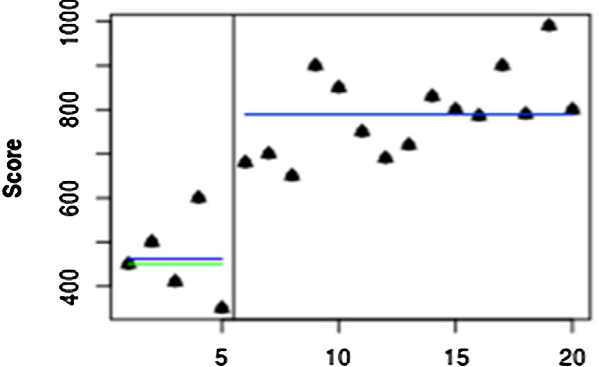 ] ] .right[ .small[For source and further information on effective visual plots see <a href="https://pubmed.ncbi.nlm.nih.gov/29253607/">(Krasny-Pancini & Evans, 2018)</a>. ]] ] <!--Trend-Lines Design--> .panel[.panel-name[Trend Lines] .small[ .pull-left-narrow[ There are various methods for plotting trends: - Split-middle trend line: Draw line connecting the median of each half phase. - OLS regression trend line: Line drawn based on regression equation for each phase. ]] .pull-right-wide[ ### .center[Trend Lines.] .center[ 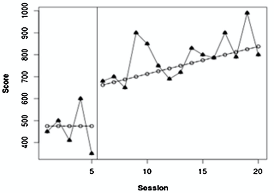 ] ] .right[ .small[For source and further information on effective visual plots see <a href="https://pubmed.ncbi.nlm.nih.gov/29253607/">(Krasny-Pancini & Evans, 2018)</a>. ]] ] <!--Trend-Bands--> .panel[.panel-name[Trend Bands] .pull-left-narrow[ Suggested that trend lines only represent the data if 80% of the data points fall within envelope bands around the trend line.] .pull-right-wide[ ### .center[Trend Lne Stability Bands.] .center[ 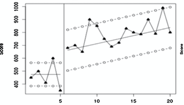 ] ] .right[ .small[For source and further information on effective visual plots see <a href="https://pubmed.ncbi.nlm.nih.gov/29253607/">(Krasny-Pancini & Evans, 2018)</a>. ]] ] <!--Stability-Lines--> .panel[.panel-name[Stability Lines] .pull-left-narrow[ Calculate the mean and SD of each phase and then draw bands 2 SD above and below the mean. Expand the bands into the comparison phase.] .pull-right-wide[ ### .center[Stability Band Lines] .center[ 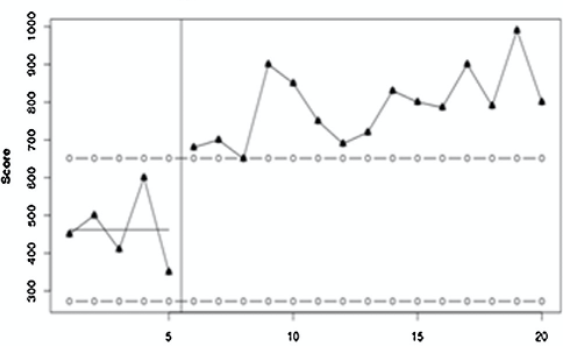 ]] .right[ .small[For source and further information on effective visual plots see <a href="https://pubmed.ncbi.nlm.nih.gov/29253607/">(Krasny-Pancini & Evans, 2018)</a>. ]] ] ] <!--Panel-Set-End--> --- # Interpreting visual plots + How much overlap between data points in each phase? + Less overlap = more likely to be differences between phases i.e. an effect! + Smaller variability within phases = easier to detect effects + Few overlapping data points between phases = intervention has had an effect. + Lots of overlap between data points in the two phases = minimal effect of intervention  --- background-image: url(images/criteria.png) background-size: contain .footnote[ Source: <a href="https://academic.oup.com/jpepsy/article/39/2/124/884297">Cohen et al (2013)</a>. ] --- # Interpreting baseline trends .pull-left-narrow[.small[ - Baseline may not be stable. Always need to interpret intervention phase in the contxt of baseline trend. - Statistics allows us tto assess and adjust for baseline trends (more on Tau-U later) ]] .pull-right-wide[  ] .footnote[For source click <a href="https://www.sjsu.edu/people/fred.prochaska/courses/ScWk240/s1/ScWk-240-Single-Case-Designs-Slides-Week-8.pdf">here</a>. ] --- background-image: url(images/base-trends-2.png) background-size: cover --- name: analysis-slide class: inverse, middle, center # Statistical Analysis --- layout: true background-image: url(uos.png), url(pearls.jpg) background-position:5% 95%, 98% 96% background-size: 110px 50px, 10% --- ## Idiographic outcomes Visual interpretation can be subjective so accompanying statistical analysis can aid interpretation. .my-red[However] need to be aware; + Can be influenced by number of time points/length of baseline + Can be misleading if there is baseline trend + Often difficult to compare + No consensus on best statistical approach/effect size metrics + Statistically significant changes may not have clinical significance + Assumptions of many statistical tests are violated in time-series data (lack of independence caused by autocorrelation ) --- # Autocorrelation Autocorrelation (also known as serial dependence) is: .my-red[The degree of similarity between one data point in a time series and a previous lagged time point i.e. how correlated are the data points.] E.g., the weather is autocorrelated: the noon temperature on a Wednesday is predicted by what the noon temperature was on Tuesday, and to a lesser extent what the noon temperature was on Monday, or Sunday. Time series data is often autocorrelated. A persons behaviour/thoughts/feelings are not random from day to day so the data is not strictly independent + Statistical tests often based on the assumption that data are independent. + When autocorrelation is present this assumption is violated (increases risk of Type 1 error [false positive]) --- # SCED effect sizes #### Metrics for capturing between phase differences + Nonparametric (overlap) and parametric (SMD, LOR etc.) + Historicaly - simple, yet commonly used overlap statistics highly criticised (e.g., PND) + More recently developed overlap effect sizes have improved (e.g. NAP, Tau) Good practice to calculate more than one overlap metric Remember they are relative to whether the desired direction of improvement is shown by an increase or decrease in the measure + Desired outcome is .my-red[increase:] intervention data points that are higher than the baseline. + Desired outcome is .my-red[decrease:] intervention data points that are lower than the baseline. --- # Non-overlap effect sizes <table class="table" style="font-size: 10px; margin-left: auto; margin-right: auto;"> <thead> <tr> <th style="text-align:left;"> Common effect sizes </th> <th style="text-align:left;"> Description *(if an increase is the direction of improvement) </th> <th style="text-align:left;"> By hand </th> </tr> </thead> <tbody> <tr> <td style="text-align:left;"> Percentage exceeding the median (PEM) </td> <td style="text-align:left;"> Proportion of observations in phase B that improve upon the median of phase A. </td> <td style="text-align:left;"> Yes </td> </tr> <tr> <td style="text-align:left;"> Percentage of non-overlapping data (PND) </td> <td style="text-align:left;"> *Proportion of observations in the B phase that exceed the highest observation from the A phase. Severe limitations as influenced by no. of time points in the baseline. </td> <td style="text-align:left;"> Yes </td> </tr> <tr> <td style="text-align:left;"> Percentage of all non-overlapping data (PAND) </td> <td style="text-align:left;"> *Proportion of observations remaining after removing the fewest possible number of observations from either phase so that the highest remaining point from the baseline phase is less than the lowest remaining point from the treatment phase. </td> <td style="text-align:left;"> Yes </td> </tr> <tr> <td style="text-align:left;"> Nonoverlap of all pairs (NAP) </td> <td style="text-align:left;"> *Proportion of all pair-wise comparisons where the treatment phase observation exceeds the baseline phase observation, with pairs that are exactly tied getting a weight of 1/2. </td> <td style="text-align:left;"> No </td> </tr> <tr> <td style="text-align:left;"> Improvement rate difference (IRD) </td> <td style="text-align:left;"> The robust phi coefficient corresponding to a certain 2×22×2 table that is a function of the degree of overlap between the observations each phase </td> <td style="text-align:left;"> No </td> </tr> <tr> <td style="text-align:left;"> Tau/Tau-U </td> <td style="text-align:left;"> Tau provides an effect estimate that does not make any adjustments for baseline trend. Tau-U is similar to Tau but includes an adjustment for baseline trends. </td> <td style="text-align:left;"> No </td> </tr> </tbody> </table> --- layout: false class: inverse .panelset[ .panel[.panel-name[Non-overlaps] <!--Front--> .small[.pull-left-narrow[ ]] .pull-right-wide[ ] ] .panel[.panel-name[PND] <!--PND--> .small[.pull-left-narrow[ # Percentage of non-overlapping data]] .pull-right-wide[ .center[]] .right[.small[Original article = <a href="https://journals.sagepub.com/doi/pdf/10.1177/0145445511399147?casa_token=00pxUhWx0BwAAAAA:aFyCI-2bXjdfSEg94bRoHvkRAXMNs71Np3IgUbsSey2QRHFC3BmPUozeMOMBAWiPIA53Vm230g">(Parker et al., 2011)</a>]] ] <!--PEM--> .panel[.panel-name[PEM] .pull-left-narrow[ .small[.pull-left-narrow[ # Percentage of data exceeding the medium]] ] .pull-right-wide[ .center[]] .right[.small[Original article = <a href="https://journals.sagepub.com/doi/pdf/10.1177/0145445511399147?casa_token=00pxUhWx0BwAAAAA:aFyCI-2bXjdfSEg94bRoHvkRAXMNs71Np3IgUbsSey2QRHFC3BmPUozeMOMBAWiPIA53Vm230g">(Parker et al., 2011)</a>]] ] <!--PAND--> .panel[.panel-name[PAND] .pull-left-narrow[ # Percentage of all non-overlapping data ] .pull-right-wide[ .center[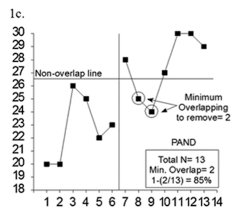]] .right[.small[Original article = <a href="https://journals.sagepub.com/doi/pdf/10.1177/0145445511399147?casa_token=00pxUhWx0BwAAAAA:aFyCI-2bXjdfSEg94bRoHvkRAXMNs71Np3IgUbsSey2QRHFC3BmPUozeMOMBAWiPIA53Vm230g">(Parker et al., 2011)</a>]] ] <!--NAP--> .panel[.panel-name[NAP] .pull-left-narrow[ # Non-overlap of all pairs ] .pull-right-wide[ .center[ .center[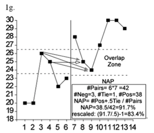]] ] .right[.small[Original article = <a href="https://journals.sagepub.com/doi/pdf/10.1177/0145445511399147?casa_token=00pxUhWx0BwAAAAA:aFyCI-2bXjdfSEg94bRoHvkRAXMNs71Np3IgUbsSey2QRHFC3BmPUozeMOMBAWiPIA53Vm230g">(Parker et al., 2011)</a>]]] ] <!--Panel-Set-End--> --- layout: true background-image: url(uos.png), url(pearls.jpg) background-position:5% 95%, 98% 96% background-size: 110px 50px, 10% --- # Example: Percentage exceeding the median (PEM) + Calculate median of baseline + =3 + Count number of intervention phase datapoints that are above the median + =37 out of 42 + Convert to a % + 37/42*100 = 88.10% PEM=88.10%  --- # Example: Percentage of all non-overlapping data (PAND) + Count how many extreme datapoints would need to be removed to there is no overlap + =6 (red circles) + Convert to % + 6/63*100=9.52% + Take the inverse + 100-9.52=90.48% PAND=90.48%  --- # Interpreting non-overlap effect sizes Effects are provided as a proportion (or *100 to make a %) The larger the effect size, the more effective the treatment .my-red[No agreed] way to interpret effect sizes but Scruggs & Mastropieri (1998) suggested the following interpretation; + 0.90+(or 90%) indicative of a very effective treatment + 0.70-0.89 (or 70-89%) represent moderate effectiveness + 0.50-0.69 (or 50-69%) are debatably effective + <0.50 (50%) are regarded as not effective --- # Tau/Tau-U for baseline trend Tau/Tau-U family of effect sizes calculates overlap with adjustments for baseline trend and is robust to serial dependency (autocorrelation). If baseline data is stable (for time series data) then Tau (τ AvsB) is a sufficient index of outcome. If there is significant trend then use Tau-U (τ AvsB-Atrend ). so first assess whether there is a significant trend in the baseline phase (Tau trend A). If there is a significant baseline trend (p<.05) then adjust using Tau-U. Dont do this by hand! - Online Tau calculator: http://ktarlow.com/stats/tau OR - Shiny apps: https://manolov.shinyapps.io/Overlap/ --- # Comparing multiple phases If you have more than two phases (i.e. any design other than A/B) then do pairwise comparisons for each bi-phasic combination of interest. In example of AB-F/U design: + Baseline (A) vs intervention (B) + Baseline (A) vs follow-up (FU) + See example published papers of different designs in your pack  --- # Assessing nomothetic outcomes Does pre/post phase scores on nomothetic measures meet criteria for reliable and clinical significant change (Jacobson & Traux, 1991)? 1. Has the client shown a .my-red[reliable change] (RC)? + Reduction in scores beyond that which could be due to measurement error. + The RC threshold will be published for most widely used measures. + If there isnt one then this can be calculated! Use the reliability (Cronbach’s Alpha) of the measure and non-clinical and clinical norms to calculate the RC. 2. Has the client shown .my-red[clinically significant change]? (CSC) + Moved from above to below a clinical cut-off threshold. + Use defined cut-off’s (if available) or calculate using clinical and non-clinical norms. + Process or generalisation measures may not make conceptual sense to assess clinically significant change (e.g. activation or quality of life). An Excel workbook & manual is provided in the Resource Pack that will allow you to do this! --- # Evaluating nomothetic outcomes using reliable & clinically significant change + Nomothetic measure of general distress: CORE-OM + Connell et al (2007) paper reports psychometric evaluation including; + Reliability of the measures (Cronbach’s Alpha = 0.91) + Clinical and non-clinical norms (mean & SD) + Established reliable change and clinical cut-off thresholds + Pre-post change >= 6 shows Reliable Change + Pre-post score moving from above to below 10 shows Clinically Significant Change .pull-left[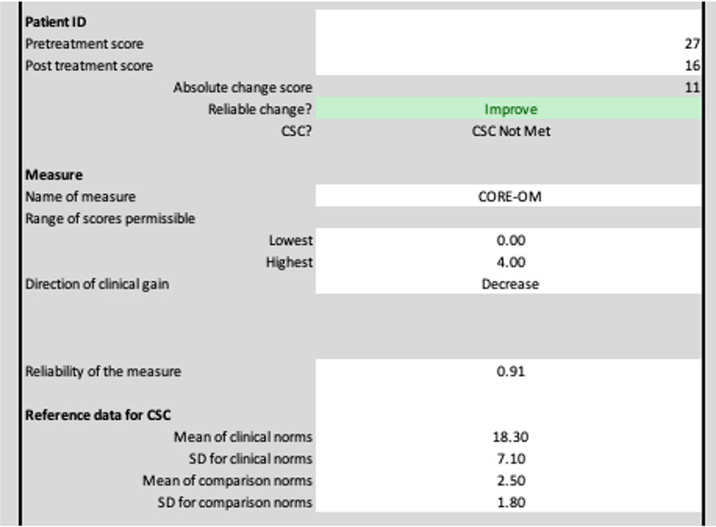] .pull-right[] --- # What do you need to include in your assignment? 1. .bold[Visual analysis:] + Visual plots of every idiographic measure. + Include phase trend lines and baseline median line. 2. .bold[Summary descriptives:] + Report means & SDs for each idiographic measure in each phase 3. .bold[Statistical analysis:] + Assess for baseline trend (appropriate Tau correction if trend is present) + Report at least 3 non-overlap statistics + Assess autocorrelation in data (instructions provided in resources). 4. .bold[Nomothetic outcomes:] + Calculate whether RC and CSC have occurred for the primary nomothetic measure. + For the other nomothetic measures calculate RC and if relevant, calculate CSC. --- # Deciding what software to use Data input and management: MS Excel Lots of the analysis can be done by hand (if you want!) More sophisticated techniques require software/web calculators (they will also do the simpler analyses/visualisation as well!) See SingleCaseSoftware table (next slides) for summary of some of the available programs/web calculators for SCED analysis. + What you can do in each program + Benefits and limitations of each program + Complexity to learn --- # Quick intro to SCED software + Microsoft Excel + Tau online calculator: http://ktarlow.com/stats/tau/ + Jepusto Shiny app: https://jepusto.shinyapps.io/SCD-effect-sizes/ + SCDA Shiny app: https://tamalkd.shinyapps.io/scda/ + Overlap Shiny app: https://manolov.shinyapps.io/Overlap/ [http://ktarlow.com/stats/tau/](https://jepusto.shinyapps.io/SCD-effect-sizes/) [https://jepusto.shinyapps.io/SCD-effect-sizes/](http://ktarlow.com/stats/tau/) [https://tamalkd.shinyapps.io/scda/](https://manolov.shinyapps.io/Overlap/) [https://manolov.shinyapps.io/Overlap/](https://tamalkd.shinyapps.io/scda/) --- layout: false background-image: url(images/software.png) background-position: 50% 50% background-size: 1200px 680px --- background-image: url(images/resource-pack.png background-position: 50% 85% background-size: 1000px 500px # SCED Resource Pack --- name:practice-slide class: inverse, center, top # Practical task .left[.white[ We will divide you into groups of 4 Two example datasets – each group will be assigned a dataset either Adult mental health setting (AB-F/U) OR Adult inpatient setting (AB) Each has a guide to walk you through conducting and reporting the analysis in different types of software There are multiple idiographic measures – you don’t have to do all of them in the practical – the examples are provided so you have a guide for the full analysis process you will need to do for your assignment + You may want to divide the measures up between your group ]] --- # Feedback your findings Present informal overview of findings (~5-10 mins per group). PowerPoint template provided to copy and paste your results into. Things to report on; - Visual plot of each idiographic measure - Assess whether there is a baseline trend using Tau/Tau-U - Calculate x3 non-overlap statistics (Tau/Tau-U counts as one!) - Descriptive statistics for each phase (means and SDs) - RCSI analysis of nomothetic outcomes Don’t worry too much about having a detailed interpretation! + This is about practicing, troubleshooting any becoming familliar with the resources. + Each dataset has a summary of the results so you can sense check if you have produced the same findings – just don’t cheat! --- # Feedback + How did you find using the different SCED software? + Any problems? + Any questions/queries? + Anything you are concerned/unsure about? --- name: last-slide # References + Cohen et al (2013) Single-Case Research Design in Pediatric Psychology: Considerations Regarding Data Analysis. Journal of Pediatric Psychology, 39, 124-127. + Krasny-Pacini & Evans (2018) Single-case experimental designs to assess intervention effectiveness in rehabilitation: A practical guide. Annals of Physical and Rehabilitation Medicine, 61, 164–179